Calculating the Astronomical Unit

during a Transit of Mercury

using Satellite Data

Dr. Sten Odenwald (NASA/IMAGE)

Dr. Bart DePontieu (Lockheed Martin/TRACE)

Suppose you were trying to measure the width of a canyon from your side to the distant canyon wall. You couldn't pace the distance. Could you come up with a way to make this measurement safely?

Surveyors and geologists encounter this kind of problem measurement problem all the time. Over the course of centuries they have found a simple way to solve this problem. They use a method called 'triangulation'. Here's how it works:

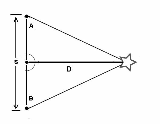
In ordinary land surveying, imagine a distant mountain peak (the star in the figure above) and two observers are located at 'A' and 'B' separated by a few miles (the length 'S'). The base angles at A and B can be measured with an instrument called a theodolite. By knowing the base distance A to B, and the baseline distance S, the distance to the peak can be worked out with a simple scaled drawing or with trigonometry.

Suppose it was hard for you to measure the two base angles in the triangulation method. This could easily happen if the object were so far away that your instrument could not accurately discern that these angles were different than 90 degrees. For example, if the object is 10 miles away, and your baseline is only 5 feet long, the two base angles would have a measure of 89.9946 degrees. This angle differs from 90 degrees by only 0.0044 degrees which equals 16 seconds of arc (there are 60 minutes or arc/degree x 60 seconds of arc/minute of arc = 3600 seconds of arc per degree!) This would be a very difficult angle to measure even with very expensive modern surveying equipment!

To solve this problem, astronomers don't bother measuring the base angles at all. Instead, they measure the vertex angle in the triangle. It turns out that this angle is very easily measured using photographic techniques. The method is called trigonometric parallax or just 'parallax' for short. Here's how it works:

Extend your arm in front of you, hold your thumb up, and alternately open and close your eyes. You will see your thumb's position move against the more distant background in front of you. Astronomers call this the parallax shift as the figure below illustrates:

But this same principle applies to measuring distance to objects far away from you too...like the planets. Today, astronomers use photographs of stars taken 6 months apart. During that time, Earth has traveled from one side of its orbit to the other, and the orbit baseline is twice 93 million miles (150 million kilometers). By measuring how far the image of a star has shifted relative to the far more distant stars in the background between, say, January and June, astronomers can accurately measure angles as small as 0.001 seconds of arc or 0.0000003 degrees.

Believe it or not, long before the time when photography had been invented, astronomers were using the parallax technique to measure the distances to the nearby planets. By the time of Kepler in the early 1600s, astronomers knew exactly how far the planets were from the sun in terms of the distance from earth to Sun, but they didn't know exactly how many kilometers this distance equaled. Instead, they had a table that looked something like this:

When you make a scale model of the solar system with its nine planets, how do you know that in this model, the actual distance from Sun to Earth is 93 million miles and not, say, 153 million or 23 million? At the time of Kepler, the best estimates for this distance were as small as 5 million miles! The answer is that you have to come up with a way to actually measure this distance. Just like land surveyors surveying a distant canyon wall, you can't travel across distance to make this measurement.

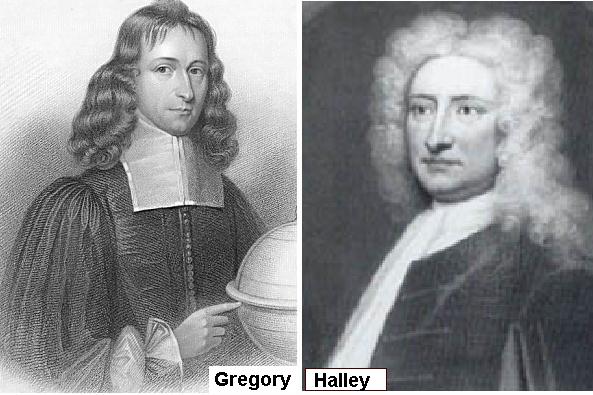
In 1663, Rev. James Gregory who was an astronomer and mathematician considered, suggested that a more accurate measurement of the Earth-Sun distance could be made. He showed how this distance could be measured from observations of the transit of Venus made from various widely separate geographical locations.  A few years later, Sir Edmund Halley, made the same suggestion in 1677, and published the details of this technique in 1716. Sir Edmund Halley described in detail how scientists from various nations could observe the upcoming 1761 and 1769 transits of Venus from many parts of the world. From the parallax shifts they would measure, they would be able to measure this distance from the Earth to Venus and the sun with near-perfect accuracy. 

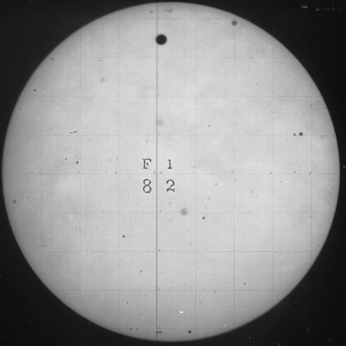
The astronomical event called the transit of Venus happens because Venus orbits the sun inside the orbit of Earth. This means that every once in a while, Venus will pass across the face of the sun. The following photograph taken in 1882 by the U.S. Naval Observatory shows what this looks like. You can see Venus as a very large black spot directly above the center of the sun's disk. The other spots in the photograph are defects and blemishes in the glass photographic plate.

When these rare transit observations were made between 1761 and 1882, hundreds of scientists were involved in dozens of expeditions to the far corners of the world to set up sensitive equipment at a cost of millions of dollars. Some scientists actually died, or were arrested, in obtaining these measurements. Thanks to modern NASA space technology, we can re-do these transit of Venus parallax measurements very simply, so that students can get an idea of how parallax works. What we will do is to use NASA spacecraft data, instead of equipment on the ground.

The TRACE satellite orbits Earth and has its sensors trained on the surface of the Sun to search for solar flares. The changing perspective of the location of Mercury in its orbit also leads to a parallax shift. Here is a close-up of the consecutive images of Mercury as it traveled across the sun on May 7, 2003:

The composite shows the position of Mercury roughly every 450 seconds.

The first method we can use is to examine a table that lists the angular shift of the disk of Mercury at various times during the transit. At the moment that the satellite captured each image of Mercury in the montage above, it was also able to measure the vertical 'North-South' shift of the center of each image every 450 seconds. The Mercury Parallax Table shown below gives the times, and the angular shifts of the centers of each image in the sequence.

Step 1..Have the students identify the largest positive (northward) and largest negative (southward) shift of the images. The answer should be +0.0046 and - 0.0044 degrees.

Step 2...Compute the difference between the largest positive and negative displacements to obtain the vertex angle. The answer should be 0.0046 - (-0.0044) = 0.0090 degrees.

Step 3...Determine the diameter of the TRACE orbit in kilometers as follows:

From the TRACE satellite orbit data at the time of the transit on May 9, 2003 the satellite was in a polar orbit (the red line in the figure below) with an altitude above Earth's surface of 580 kilometers.

Step 4: Now that we have determined the vertex angle from Step 2 and the orbit radius, R, from Step 3, we can use the formula:

to determine the distance from Earth to Mercury (D). First, solve this equation for D:

 At the time of the transit on May 7, 2003, the distance between the Earth and Mercury was predicted to be 0.56 Astronomical Units. To find our estimate for the Astronomical Unit, we use the proportion: 1.0/L = 0.56/ D. Solving for L, this means that

We can also use the TRACE Mercury Transit image to determine the distance to Mercury. To do this, we first have to determine the scale of the print so we can measure the parallax angle q. 

Step 4: At the time of the transit, the angular diameter of the sun is known by astronomers to be 0.53 degrees (1903 arcseconds) . Calculate the scale of the solar circle in degrees per millimeter by dividing 0.53 degrees by the measured diameter of the sun circle (210 millimeters) . Call this number 'A'. A value near 0.0025 degrees per millimeter is appropriate.

A simpler, though less accurate, method is to use the astronomical fact that the diameter of Mercury in this image is 0.0033 degrees (12 arcseconds) , and use this to calculate the scale of this image.

Step 8: Calculate the vertex angle, P, in degrees by using the formula P = A x S. In the example, P = (2.0 mm) x (0.0026 deg/mm) = 0.0052 degrees. In the diagram for the parallax geometry, the vertex angle, P, is twice as large as the parallax angle q so that q = 0.0026 degrees.

Step 9: The TRACE satellite obtained the Mercury images by first shifting the solar disk image to the center of the picture frame, then taking the 'picture'. Since the solar image was re-centered each time, this solar parallax was subtracted from the full parallax angle we need to measure. To recover this 'instrumental effect' in the data, you have to add back the 0.0019 degrees for the spacecraft repointing, to the parallax angle you measured on the image. The full Mercury parallax angle q is then 0.0026 + 0.0019 = 0.0045 degrees.

Tan (q) = R / D

From the example where the parallax angle q = 0.0045 degrees, we get a distance from Earth to Mercury, of